Documentation for Quadratic Spline Fertility Schedule Fitting
INTRODUCTION [Back to Top]
QS MODEL [Back to Top]The constrained Quadratic Spline (QS) family of fertility models is described in detail in Schmertmann (2003). Age-specific fertility rate (ASFR) schedules in the QS family have three shape parameters and one level parameter. The shape of a QS schedule depends on the initial age at which fertility rises above zero (α), the age at which fertility rates peak (P), and the first age above P at which fertility falls to half of its peak level (H). A QS schedule consists of five quadratic pieces, assembled to ensure that levels and slopes of the resulting ASFR curve are continuous, and to ensure that the ASFR curve has "good" demographic properties. See the full text for details.
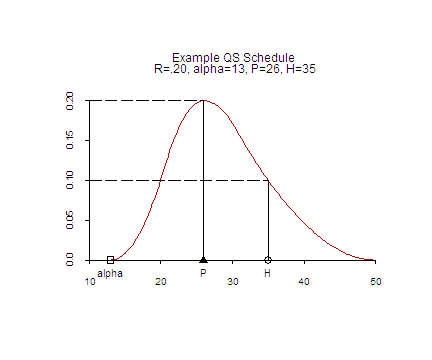 The graph to the left shows one example of a QS fertility schedule, with a shape defined by (α,P,H)=(13,26,35).
The value of R (.20 in this case) determines the height of the curve at peak age P.
The graph to the left shows one example of a QS fertility schedule, with a shape defined by (α,P,H)=(13,26,35).
The value of R (.20 in this case) determines the height of the curve at peak age P.
It is useful to think of the QS schedule as a slack line, pinned to the age axis at ages α and 50, then draped over a tall pole at age P and a short pole at age H. The height of the pole at age P is R, and the height at age H is R/2.
Changing the index ages changes the horizonal positions of the "poles" and alters the shape of the ASFR schedule accordingly. The QS family of shapes defined by these three age parameters is quite flexible and fits many empirical schedules well.
Schmertmann (2003) also suggests two behavioral indices related to QS parameters: a delay index [D=P-20] for pre-peak fertility control, and a stopping index [S=(P+50)/2-H] for post-peak control. Estimates of both D and S appear in program output.
PROGRAM [Back to Top]
The web program fits a QS model to an empirical schedule supplied by the user. It finds the (R,α,P,H) combination that minimizes the unweighted sum of squared differences between a user-specified set of empirical nfx values and the corresponding values in a QS schedule. The user types or pastes data into a text window and clicks a button to start the fitting procedure. The program produces several types of text output reports, as well as a graphical image of the empirical schedule and the QS model fit.
SCREEN LAYOUT [Back to Top]
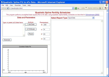
The program screen is divided into three main panels -- Data and Parameters in the top left section, Graphics on the lower left, and Reports on the right, as illustrated in the image below.
INPUT [Back to Top]
DATA ORGANIZATION [Back to Top]Input data consist of lines of text, each representing an age interval. The first value on a line is the exact age at which the interval begins; the second is the interval's fertility rate. For each interval except the last, the ending age equals the starting age on the next line. The last interval always ends at age 50.
For instance, clicking one of the
 buttons automatically enters text lines of example data: a 2002 period 5fx schedule for Iran (Example 1),
or a 1996 period 1fx schedule for Sweden (Example 2).
buttons automatically enters text lines of example data: a 2002 period 5fx schedule for Iran (Example 1),
or a 1996 period 1fx schedule for Sweden (Example 2).
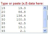
In the case of the Iranian data in Example 1, the text is:
15 19.3
20 86.8
25 136.4
30 100.5
35 42.5
40 15.1
45 2.1
and the program interprets these data as an ASFR schedule for seven standard five-year groups, 15-19...45-49. Age intervals can be any width, and the intervals can be different widths. (Each interval receives equal weight in the fitting procedure, however, whether or not their widths are identical.)
DATA ENTRY [Back to Top]
Enter data in the data pane:
either by typing x and f values directly as text, by cutting and pasting data from other applications such as spreadsheets, or by a combination of these techniques. Ages and rates can be separated with commas, spaces, or tabs. If there are more than 7 lines of data, the window will scroll appropriately. Note that the program always interprets periods [ . ] as decimal points, and commas [ , ] as separators between x and fx values.
After entering data lines, click
 to load the empirical schedule into the estimation program.
Data will load as text in the report window on the right, and also as a bar graphics panel on the lower left.
(There may be a delay in plotting if the Java applet in the lower left window is still loading.)
to load the empirical schedule into the estimation program.
Data will load as text in the report window on the right, and also as a bar graphics panel on the lower left.
(There may be a delay in plotting if the Java applet in the lower left window is still loading.)
When data are set, the program also sets starting values for the QS parameters (R, α,P,H) in the non-linear least squares (NLS) fitting algorithm. These appear in the four labeled windows on the right of the Data and Parameters panel. Parameter values are automatically updated while the fitting program runs. The automatically-defined starting values are usually adequate, but occasionally (especially if the empirical schedule is unusual) the user may need to alter them manually before starting to fit the model.
MODEL FITTING [Back to Top]
After setting the data, click
 to begin fitting. Results appear in the Report and Graphics panes.
The program searches for the set of QS parameters that minimize the unweighted sum of
squared differences between the nfx values supplied
by the user and the corresponding nfx values in a QS schedule.
to begin fitting. Results appear in the Report and Graphics panes.
The program searches for the set of QS parameters that minimize the unweighted sum of
squared differences between the nfx values supplied
by the user and the corresponding nfx values in a QS schedule.
OUTPUT [Back to Top]
PROGRAM COMPLETION [Back to Top]The nonlinear least squares search algorithm ends in one of three ways:
- Convergence (the search has found a solution)
- Failure to find an improvement (the search is stuck)
- Maximum number of iterations exceeded (the search is too slow)
An alert window informs the user which of these three situations occurred. If the search has not converged, check the data for input errors. If necessary, reload the data and manually change the starting parameter values before fitting.
GRAPHICAL OUTPUT [Back to Top]
The lower left panel plots the empirical schedule as a bar graph, and the current QS model function as a solid line:
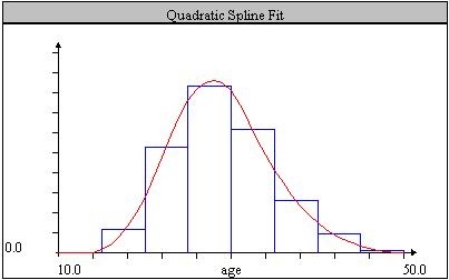
The QS plot changes with the parameter changes on each iteration of the search algorithm. On fast computers the search algorithm may be faster than the drawing algorithm. This speed difference might make QS line plots flicker while the program is running, with a clear display only for the final QS fit.
TEXT REPORTS [Back to Top]
Text output from model fitting appears in the right half of the program window. A selection bar at the top of the window allows the user to display any one of four reports:
- Input Data
- Parameter Estimation
- Observed and Predicted nfx values
- Fitted 1fx and f(x) values
button. This report is a table of x, x+n, n, and nfx values that
illustrates how the program has interpreted the fertility schedule entered by the user.
The other reports, including the Parameter Estimation report, appear automatically after a successful fit. The Parameter Estimation report begins with a history of parameter values and total squared error on each iteration of the search algorithm. For hard-to-fit schedules this iteration history may occupy most or all of the visible report pane, in which case the user must scroll down to see the rest of the report. The Parameter Estimation report also includes final estimated values of the QS parameters at convergence, together with approximate standard errors. It includes the Delay and Stopping indices derived from the final QS estimates, and also the final spline parameters and knot values used in QS calculations.
The Observed and Predicted nfx Values report gives the mean absolute error and root mean squared error of the QS model fit across age intervals, the % relative error measure described in Schmertmann (2003), and the observed (=empirical) and predicted (=best QS fit) nfx values for each interval.
The Fitted 1fx and f(x) values report displays fitted fertility rates for single-year age groups and exact ages from 10 to 50. Note that values in this report are those for the best-fitting QS model, which has only four parameters. As such the reported 1fx values will interpolate the user's empirical schedule approximately, but not exactly.
TECHNICAL DETAILS [Back to Top]
PROGRAM DESIGN [Back to Top]The web program combines HTML, JavaScript, and Java components. The overall structure and appearance come from the HTML layout. The main web program is written in JavaScript. The JavaScript program is the workhorse -- it defines the mathematical functions used in the nonlinear least squares fitting procedure, sets up the reports, and determines what actions to take in response to user inputs. The JavaScript program also drives the graphical output, via a publically available Java applet (xymeter) created in 1997 by Ralf Moros of the University of Leipzig.
Interested users can examine the HTML, JavaScript, and Java source code directly.
SEARCH ALGORITHM [Back to Top]
The web program attempts to find QS parameters (R, α,P,H) that solve a nonlinear least squares problem. Specifically,
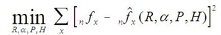
where each term in the sum corresponds to one line of data input by the user.
When the user loads data with the
button, the program parses the empirical schedule to find reasonable starting values for the four QS parameters.
Clicking
begins an iterative search, starting from the parameter values in the four windows.
On each iteration, the program calculates numerical derivatives of the objective function with respect to each parameter, and finds the search direction for the standard NLS update (e.g., Greene 1997:455). The program checks at several multiples of the standard update vector and selects the one that lowers SSE the most. If none of the tested parameter combinations in the designated search direction yield an improvement, the program performs a secondary search of 8 additional points, by changing each parameter to 90% and 110% of its current value. At this point, the program stops if none of the parameter combinations tested lowers the SSE; otherwise it selects the best combination tested and repeats the iteration.
Convergence is defined by a less than 1-part-in-10000 change between two iterations in the objective function and in all four parameter values
After convergence, the program calculates approximate standard errors, as in Greene (1997:eq 10-13). These standard errors are meaningful if the user believes that the empirical observations were drawn from process in which a QS schedule gives the true rates. Otherwise they give only an approximate idea of precision.
REFERENCES [Back to Top]
WH Greene, 1997.Econometric Analysis . Third edition. Prentice-Hall. Upper Saddle River, NJ, USA.R Moros, 1997. XY-Meter . Java source code, documentation, and compiled applet downloaded August 2004 from
http://techni.tachemie.uni-leipzig.de/jjar/jappl/xymeter/XYMeterDoc.html
CP Schmertmann, 2003. "A System of Model Fertility Schedules with Graphically Intuitive Parameters". Demographic Research 9/5.
http://www.demographic-research.org/Volumes/Vol9/5.